Contents

The Infrastructure: Loading Data and Writing Models

A few decades ago (at least that’s what it seems like) I explained AdaIn, a neural style-transfer method that I’m reimplementing for the OAK-1. I’ve finally got a model up and running, but there’s quite a lot to write about. So in this post, after a quick recap I’ll focus on loading the dataset and writing some models. The post after this one should be live in about a week or so.

Note that this post is a bit more technical than the last; you should be able to follow the rest of the project even if you skip it. Additionally, note that my goal is to go over what parts of the code are relevant to AdaIn, not to teach PyTorch from scratch.

Recap

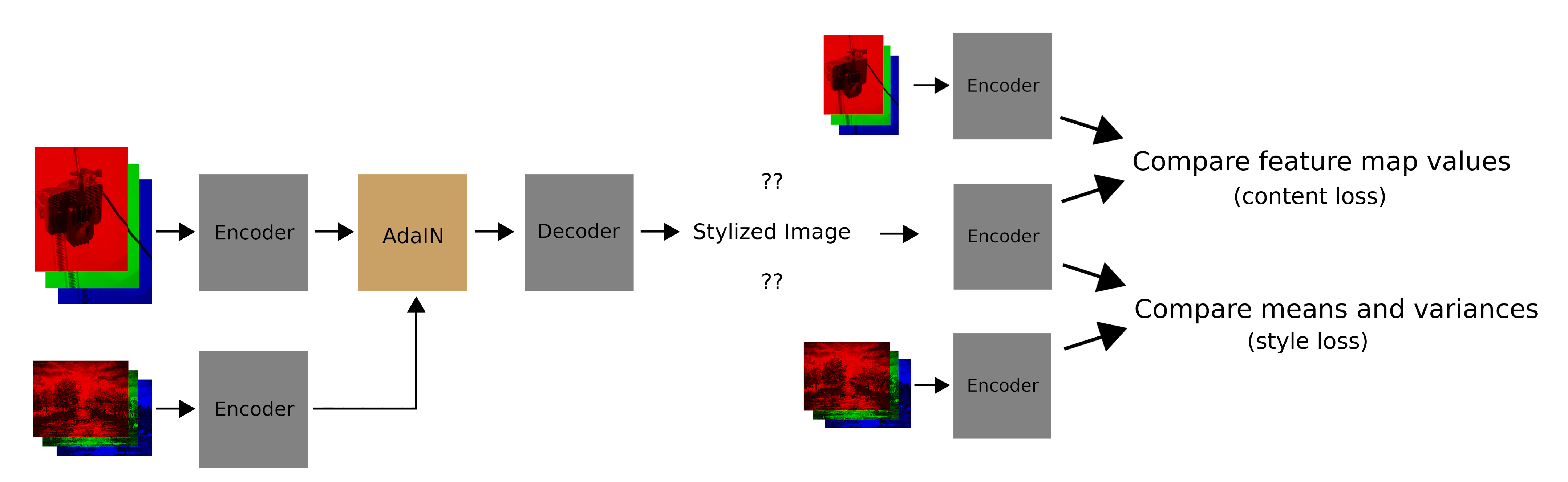
As a quick recap, here’s how AdaIn works:

1. Encode the style and content images
2. Adjust the feature-map statistics of the content encoding to match those of the style encoding
3. Decode the adjusted content encoding into a stylized image
4. Compute a style loss and content loss for the stylied image (only during training)

Here’s what this looks like if you’re a pictures person:

Loading the Datasets

First up is to download the datasets. As in the AdaIn paper, the images we’ll stylize are from the Microsoft Common Objects in Context (MS COCO) dataset, and the style images are from WikiArt. Both datasets have around 100,000 images.

MS COCO requires this API. You should be able to install it as pycocotools from pip, but if that fails, you can install it from source. I ended up installing from source. While doing so, I had to reference this issue. Additionally, I had to run make install, which I didn’t see in the instructions.

After installing the API, the COCO website recommends downloading the dataset with gsync, but that method is widely reported to be broken. Luckily, I found the datasets at these links:

Instead of using wget I used aria2 to download them, which can significantly increase download speeds (it was pretty insane).

Here’s the script I used:

The script downloads the files and moves them to a datasets directory. One thing to note is that the datasets do take up a lot of memory. Another thing to note is that I got a few errors while unzipping the files… which I ignored…

Next up was writing the dataset class. PyTorch already includes dataset classes for MS COCO, and a generic dataset class that works for WikiArt, so I leveraged those. However, technically one datapoint is a photo from MS COCO, and a painting from WikiArt. This means that a style transfer dataset’s length would be length(wikiart) * length(mscoco), or ~10 billion, which is unreasonable.

The IterableDataset doesn’t decide ahead of time which datapoints will appear, solving the issue of a dataset with 10 billion items. The IterableDataset also allows the model to always see new examples. However, it makes debugging on just a few fixed examples difficult. Another method is to pick a random fixed set of datapoints ahead of time; in this case the model wouldn’t be seeing new data, but debugging on the same few examples would be easy. I ended up implementing both methods; the former for large-scale training, and the latter for debugging.

Now lets dive into the dataset code. I’ll only explain the IterableDataset version, as I think there’s more to learn there. The whole thing is here.

This function returns the transforms we want to apply to each item in the dataset. One reason we resize is for memory efficiency. Additionally, throughout the model the dimension of the images get halfed repeatedly and then doubled repeatedly; if the dimension is ever odd before halving, then the input and output image sizes will be different, and we won’t be able to compare them. While likely unnecessary, the crop forces the model to be able to adapt more during training.

In the dataset constructor I create the MS COCO and WikiArt datasets and set the random seed used to pick new datapoints. Note that labels for coco (“coco_annotations”) aren’t necessary for style transfer, as I just need the images. However they are required as an argument to the ready-made PyTorch CocoCaptions dataset, which I wanted to reuse. The “exclude_style” flag was used when I first tested the models, as I didn’t use the style images.

The next interesting function was __iter__. This gets called before we start looping through the dataset, and for each “worker” that is preparing data in parallel. When multiple workers are used in PyTorch, the IterableDataset gets copied for each worker. So if we have four workers, four IterableDatasets will be used to prepare data in parallel.

When I check whether worker info is not None, I’m essentially checking if there are multiple workers. If there are, each IterableDataset needs to set its random state so that it doesn’t return the same datapoints as the other workers. Each IterableDataset also has to change its length; if we want a dataset of length 32 and we have four workers, each worker should return 8 items, not 32.

Next, I wrote the __next__ function, which returns the next datapoint. It checks whether the end of the dataset has been reached, and if not, returns a random image pair (or just one image, if exclude_style is True). Additionally, I have a function _check_data_to_return, to ensure that I’m returning PyTorch tensors, not PIL images or something else by accident.

That’s pretty much it for the IterableDataset class; in tests.py I wrote a test_data function to make sure everything was working.

The Encoder

For the models, I first wrote the encoder. This is a pretrained VGG19 model, with everything after the first ReLU with 512 features deleted.

I actually spent weeks trying and failing to get the whole system working because I figured I could use a VGG19 encoder that does not have batch-normalization layers. This was the one thing I had to check the original AdaIn repo for. I think unnormalized VGG19 fails because without the normalization, it’s too hard for the decoder to match feature statistics.

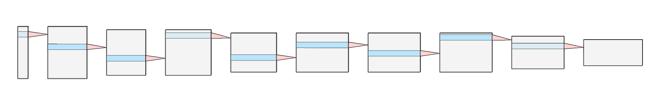
Below I’ve included a diagram of the architecture. The first gray block represents the 256x256 RGB input image, the last gray block represents the final encoding, and each blue-red arrow represents a convolutional layer. I’ve omitted activation, batchnorm, and pooling layers in the diagram.

^{Diagram made here}

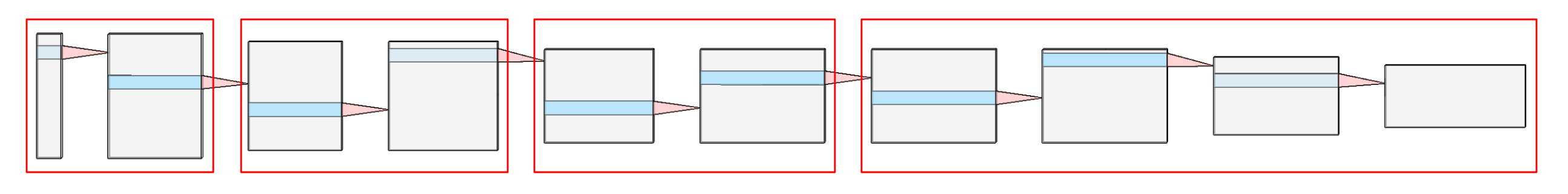
When we compute the style loss, we do so at various intermediate outputs of the encoder. In the diagram below I’ve grouped the layers into red blocks. The output at the right end of each block is used to compute part of the style loss. For example, the first red block looks like so:

convolution -> batch norm -> relu -> convolution -> batch norm -> relu

The output of the second ReLU layer feeds into the next red block, and is also used to compute the style loss.

Now let’s go through the code.

On a high level, in the constructor we load the pretrained model, switch to using reflection padding, and freeze the weights. The code for those functions is below:

I think most of this code speaks for itself. One thing to note is the weight freezing. The encoder represents what we know about natural images, so we don’t want to train this; we keep it static. We can do this by preventing the weights from calculating their gradients. We also set the model to eval() mode, so that the batch normalization settings do not get updated during training.

On the same note, the train() method by default tells the model whether it should act as if it is training mode (and thus update things like batch normalization settings), or evaluation mode. So I overrode this method, preventing myself or others from accidently using the encoder in train mode.

The rest of the functions for this class more straightforward; e.g. passing the input through the model. If you are interested, read the rest here.

I also wrote a test function for the encoder in tests.py.

The Decoder

The decoder was a little bit more complicated. It’s essentially the encoder but reversed.

Again the constructor is a high-level overview. Method load_base_architecture is a bit of a misnomer; this function loads the VGG19, but also reverses it and only takes out the layers we need. The other functions do what they say. We want to progressively grow the image size so we swap out the maxpools. Then we need to swap the direction of the now-reversed convolutional layers, and initialize their weights. Lastly, there’s a fix we need to apply to the ReLU layers (more on this later).

The method load_base_architecture loads, reverses, and truncates the VGG19 model. Method swap_maxpools_for_upsamples swaps max pooling for upsampling.

The next method, initialize_and_swap_direction_of_conv_layers, reverses all of the convolutional layers. In the original VGG19 architecture a layer might take in 256 feature maps, and output 512. Since we reversed the model, we now need that layer to take in 512 feature maps, and output 256. We also need to initialize the weights so that the model will train well; I use Kaiming Initialization, which is designed for use with ReLUs.

Lastly, make_relus_trainable sets inplace to False for the ReLU layers. When set to True, a ReLU will overwrite its input, and then return the input. The problem is, to calculate gradients, a ReLU needs to know its original inputs. In other words, we need the ReLUs not to overwrite their inputs if we want to train the decoder.

Note that we aren’t training the encoder, so we don’t have the same problem in that case.

As usual, I wrote a test function for the decoder in tests.py.

The AdaIn Layer

After writing the encoder and decoder, I tested them together for a reconstruction task. However I will save that for next post. Next is the AdaIn function.

I use PyTorch’s built in instance_norm to normalize the content encoding to zero mean and variance of one, and then shift the normalized encoding to match the means and variances of the target style-encoding.

One thing to note is that in this code I have some dimension checks to make sure I didn’t make any mistakes; these broke in early experiments with exporting the model for the OAK-1, so they will disappear later 😞.

As usual, I wrote a test in tests.py for this layer too.

Last Thoughts

And that sums up all of the core components! I actually created one more model that combines the encoder, decoder, and adain. However, I think that that model is best saved for next post, when I talk about the training pipeline. Look out for that post (and some stylized images) in the next week or so!

Previous Post Next Post

HELLO

© 2021 Antioch Sanders
Made with Jekyll