Real-time Style Transfer with AdaIN, Explained
Edited March 9th to correct loss function, which I over-generalized. Edited Aug. 24th to correct loss typo.
Recently I got an OAK-1 (a camera with an AI chip on board) and had no idea what to do with it. I also recently read the 2017 paper introducing adaptive instance normalization (AdaIN) and enjoyed it.
That’s where this project comes in. Given an input image (say a painting), I want to convert the video feed from the OAK to the style of that image. I’m not doing anything new per se, but I think it will be fun either way.
This first post will cover some basics along with the technique I’ll be using; if you’re already a deep-learning practitioner, I’d just read the original paper. In the second post, I’ll discuss re-implementing the model and training, and for the last post, I’ll move things to the OAK-1.
More on the OAK-1
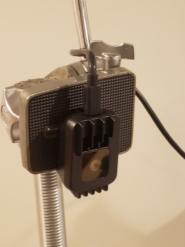
Here it is… It cost about $99 and features 4K video and an onboard neural network chip.
CNN Basics
I won’t exhaustively cover convolutional neural networks (CNNs) here, but I’ll go over enough of the basics for the rest of this project to make sense.
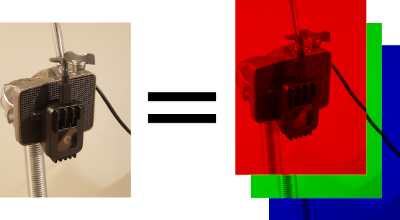
Most images are made up of 3 channels; red, green, and blue.
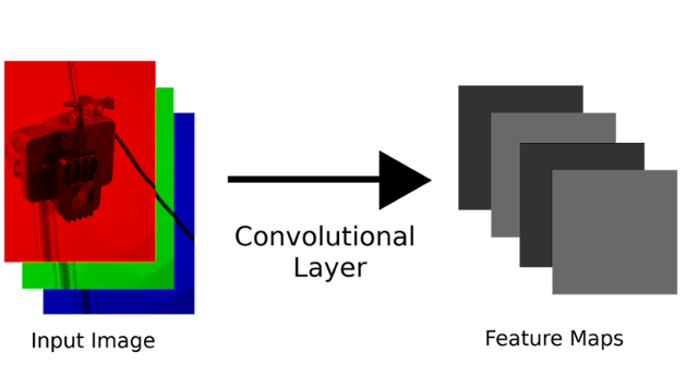
A convolutional layer is a function that takes in a stack of 2D arrays (for example, an RGB image), and transforms it into another stack of 2D arrays. So a layer might take in a 64x64 RGB image (64x64x3), and spit out four 32x32 outputs (32x32x4). Each of the four outputs is called a feature map.
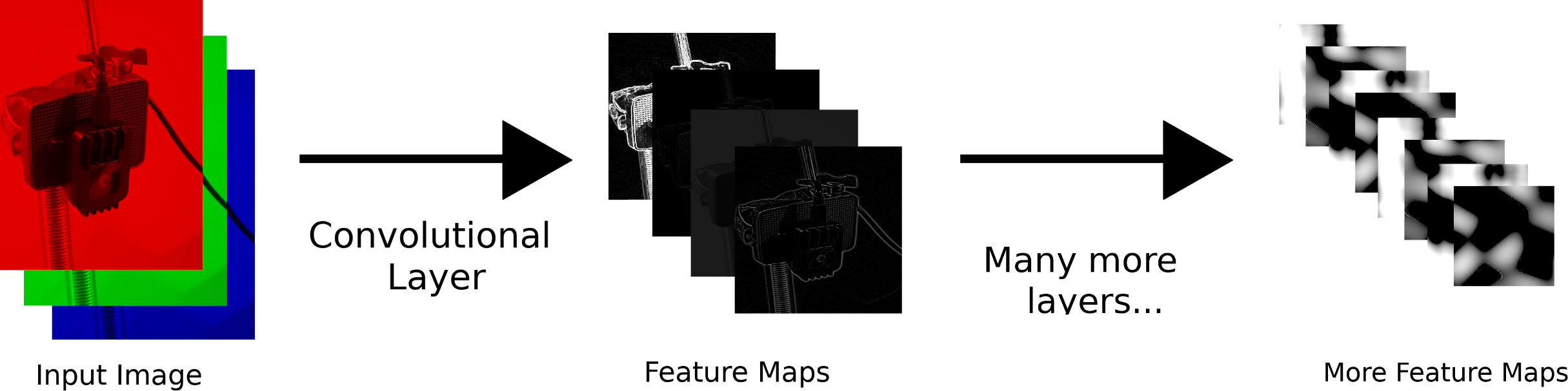
If we stack a bunch of convolutional layers together, we get a convolutional neural network (CNN). The first layers do simple things like detect lines, while later layers detect more complex patterns, like different kinds of blobs.
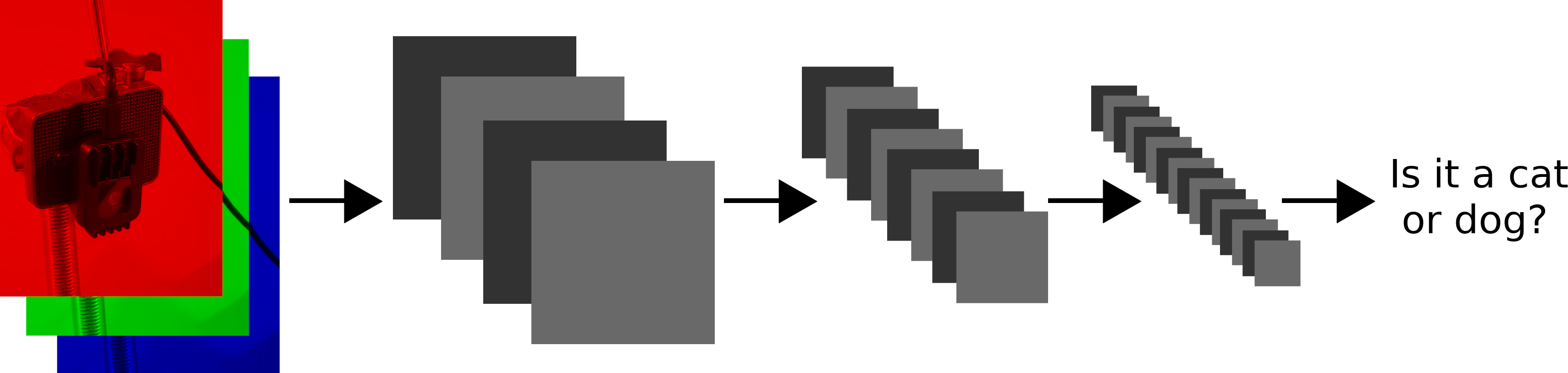
The cool thing about CNNs is that if we have enough feature maps per layer, enough layers, and lots of labeled data, we can model pretty much any function we want. For example, whether a photo is of a dog or a cat.
Encoders and Decoders
Most CNNs add more and more feature maps until they output some answer to a question we have. Here’s an example:
It just so happens that if we cut off the last few layers of a CNN, often the resulting feature maps still tell us lots of information.
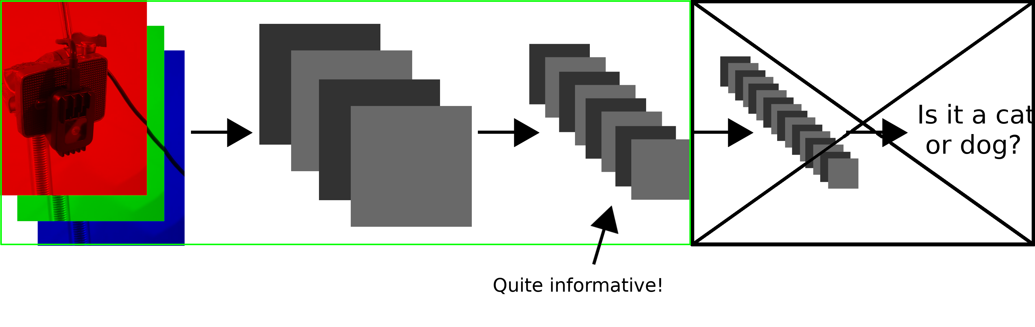
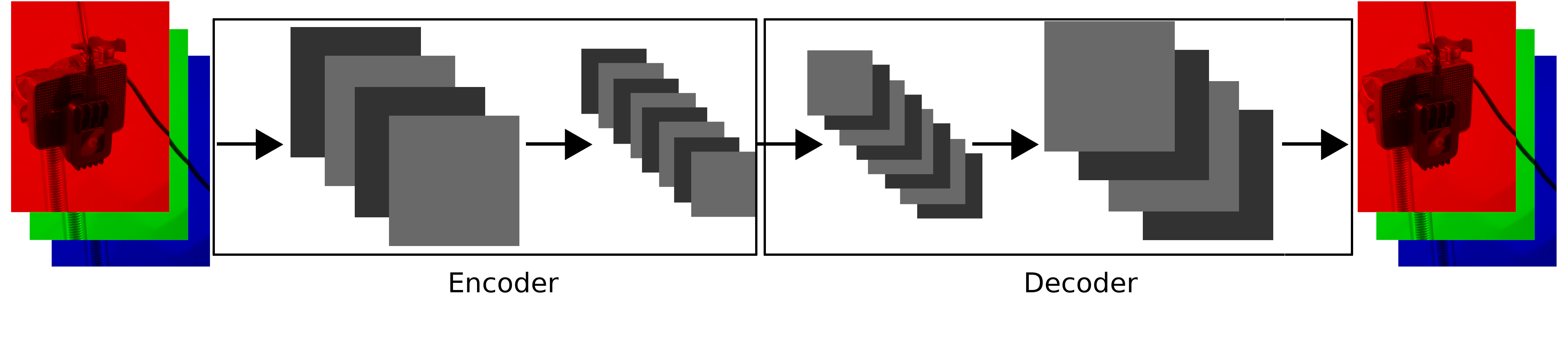
They tell us so much information that if we design a CNN that takes in these feature maps, we can train it to output the original image. We then call the first CNN an encoder, and the second CNN a decoder.
Feature Map Statistics
We’re almost there…
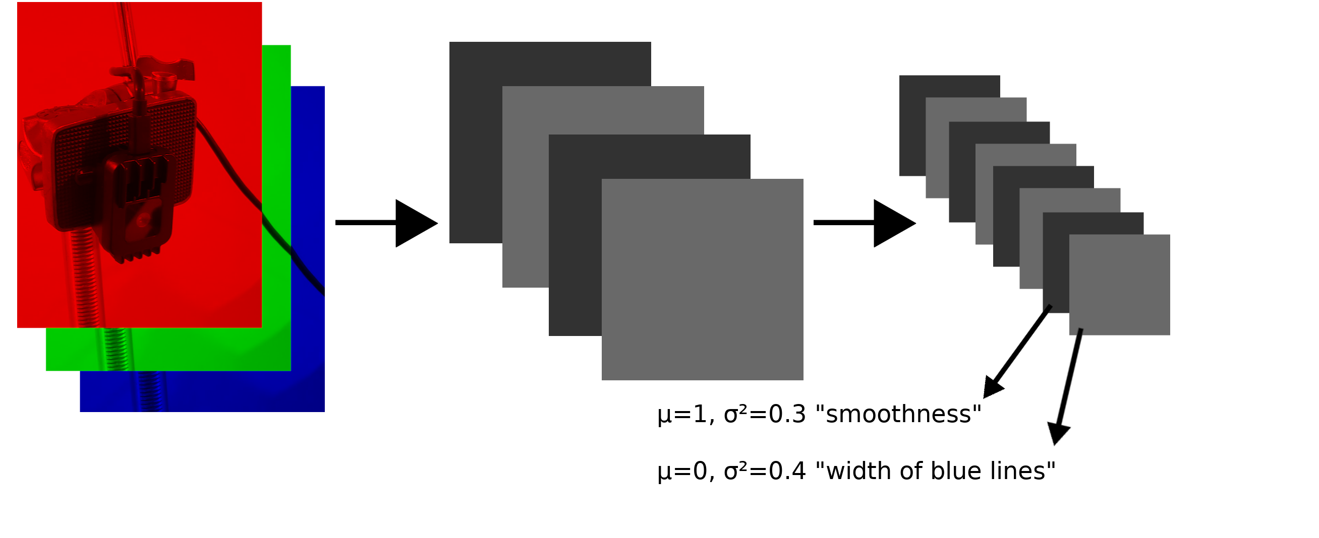
Each feature map after a convolutional layer will have an average and variance. The powerful insight made by the authors of the AdaIn paper is that these statistics tell us tons about the style of an image.
The statistics of one feature map might tell us about the smoothness of an image, while the statistics of another might tell us about the width of blue lines (this is just an example).
Let’s say we have a photograph, and after encoding it, we calculate the average and variance of each feature map. Now say we do the same with a painting.
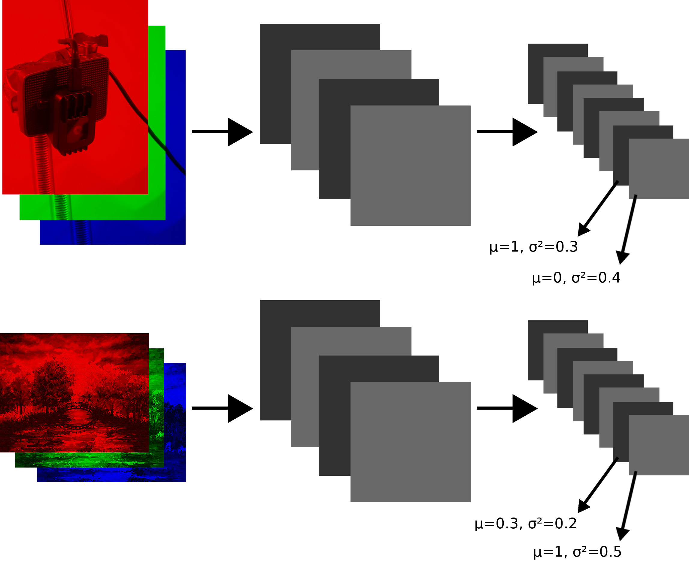
Note that the statistics of the photograph’s feature maps don’t match the statistics of the painting’s feature maps. This tells us that the images have different styles.
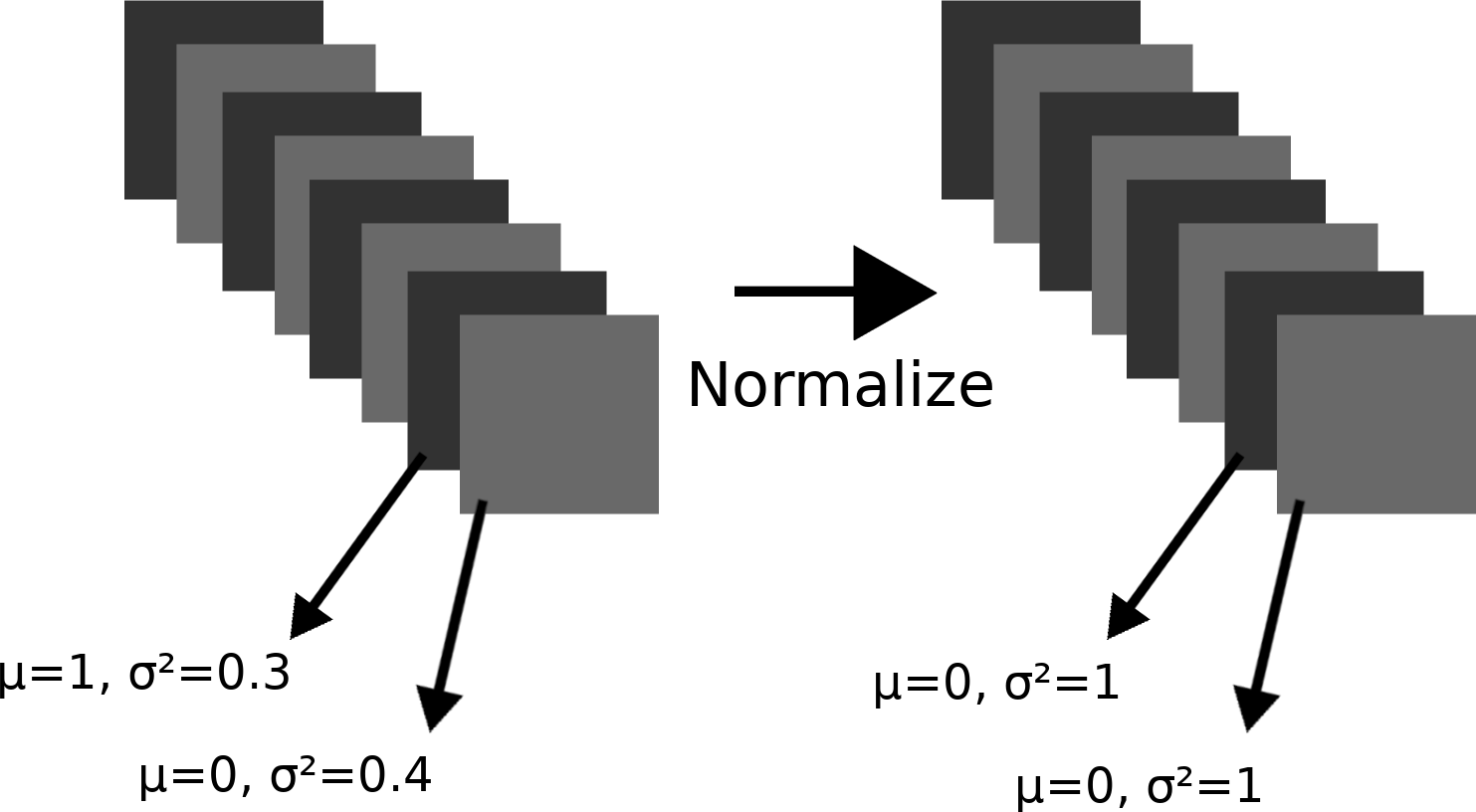
Now we can normalize each feature map of the photograph’s encoding so that each feature map has mean 0 and variance 1.
Now we can multiply by the standard deviation of the corresponding feature map in the photograph’s encoding, and add the mean of the corresponding feature map in the photograph’s encoding.
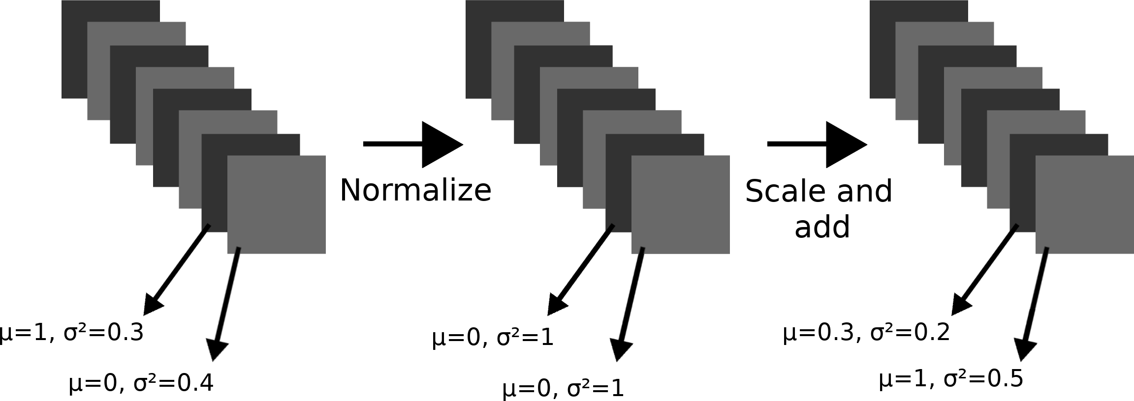
In essence, we’ve modified the photograph’s encoding so that each feature map has the same statistics as the corresponding feature map in the painting’s encoding. This step is called adaptive instance normalization, or AdaIn. The “adaptive” part comes from the fact that we can do it for any painting, and the “instance normalization” part comes from the fact that we can do it with just one input image and style image.
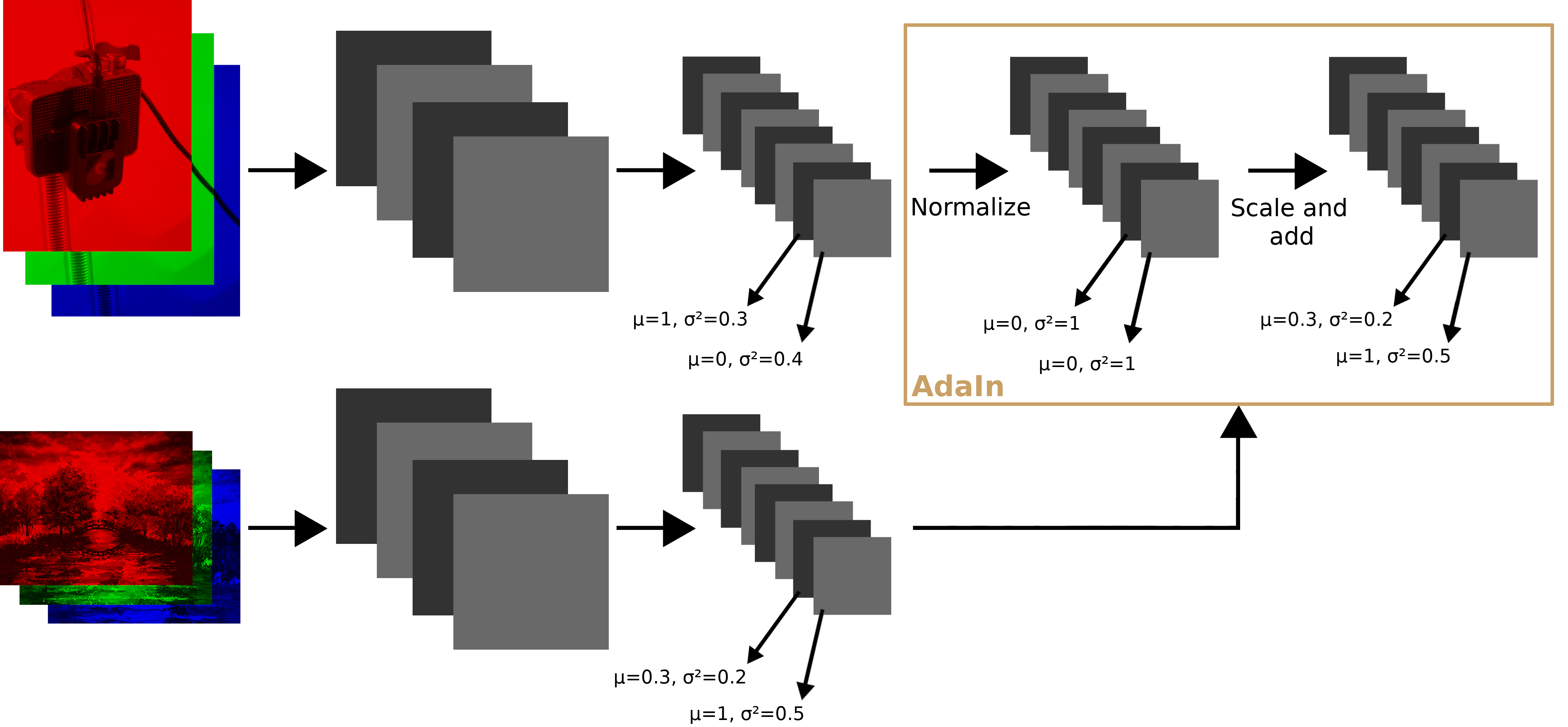
Because feature map statistics dictate the style of the image, we will get the photograph in the style of the painting after we decode the photograph’s normalized and scaled encoding.
Teaching the Network
The next question is: How exactly do we do all of this? For the encoder, we can just use a model that someone else has trained for image classification (as the AdaIn authors do), and not change what it does (its weights). But the decoder needs to be trained to reconstruct an image in a different style.
There are two things we want the decoder to do. First, the decoder should output an image that matches the target style. For this we compare feature map statistics:
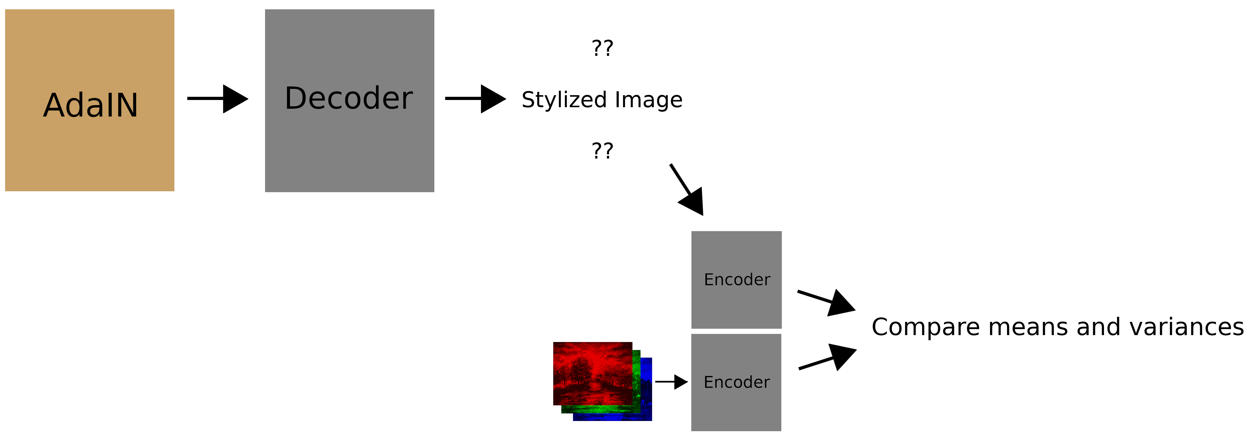
We can measure how badly the decoder is doing this numerically with the following function:
Intuitively, this calculates how far away the output style is from the style image’s style; if the target style is very smooth, the output image should be too.
Second, the decoder should output an image that matches the content of the input feature maps it was given. For this we compare the feature map values (not the statistics):
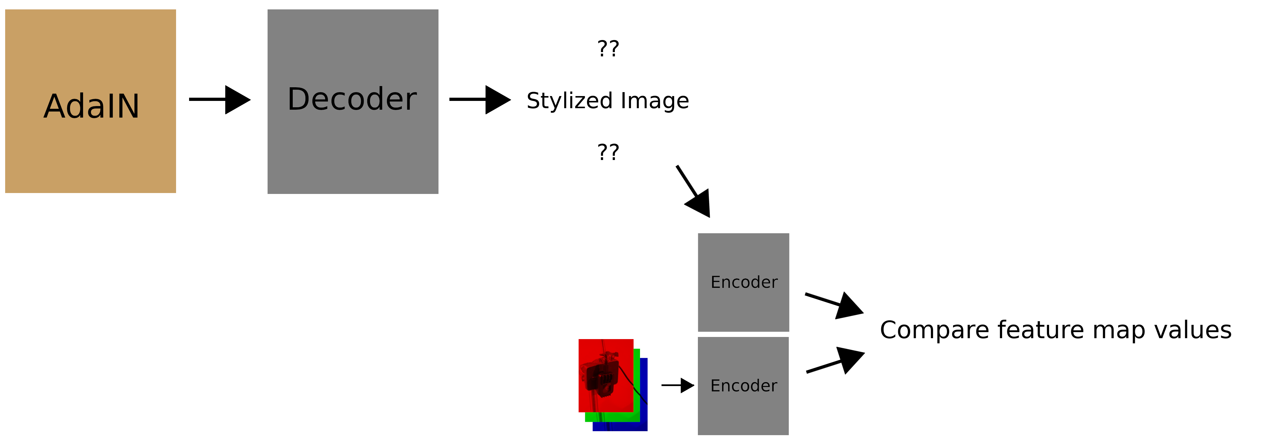
Numerically, this is:
Intuitively, this calculates how far away the output feature maps are from the feature maps of the input. In other words, a car should still look like a car.
In practice, we don’t just compute these loss functions with the output of the encoder; we use intermediate layers of the encoder too. Also, to balance the content loss and style loss, we introduce a scaling factor \(\lambda\).
This leads us to the following loss function:
We can minimize this loss function with gradient descent. That is out of the scope of this post, but I hope the idea behind what we’re trying to do makes sense.
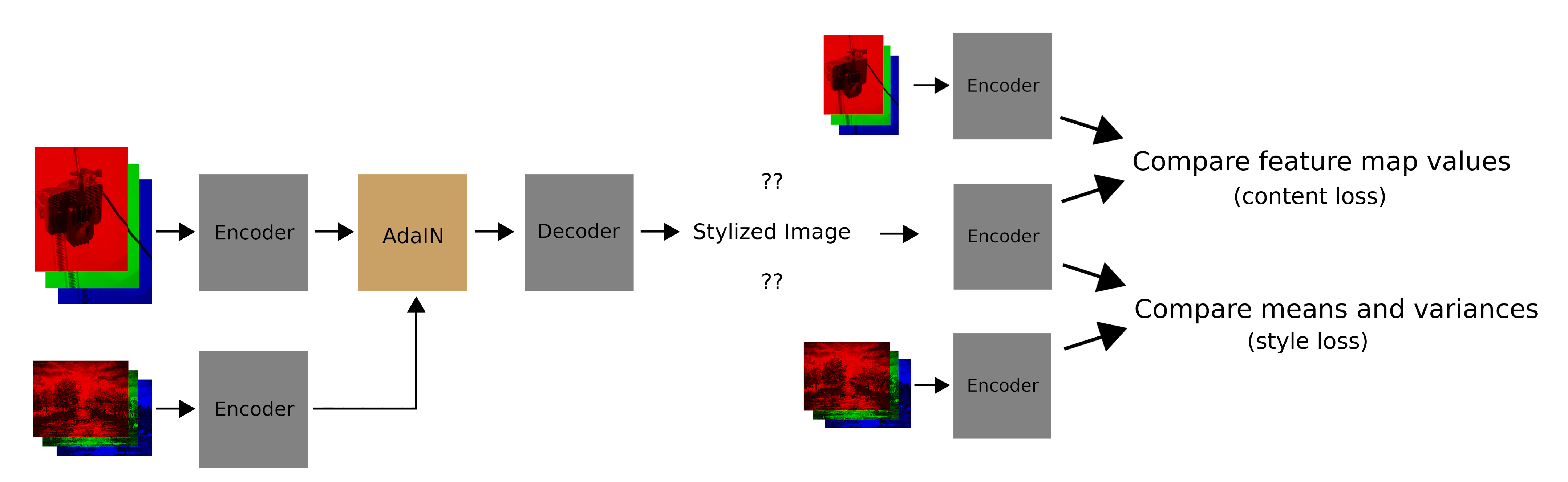
The whole system looks as follows during training:
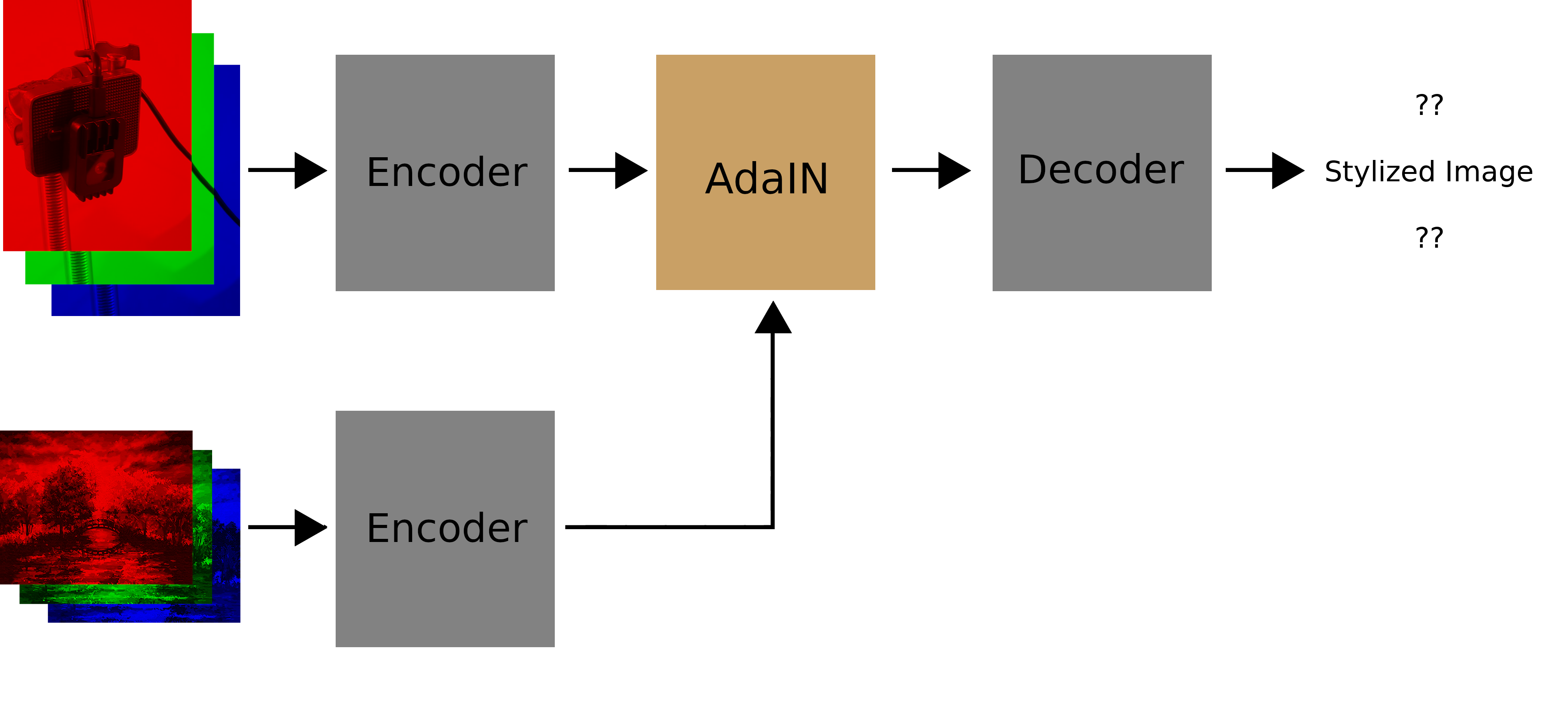
And as a recap, this is how things look when we are actually using the system:
And that’s it for now! I’ve already made quite a bit of headway on writing the models, so look out for the next update.
Example style image stolen from here.
| Back to Project |
Get occasional project updates!
Get occasional project updates!